Example of using archetypal analysis to find representative cells & describe heterogeniety in hepatocyte population between those archetypes
Vitalii Kleshchevnikov
11/01/2019
Hepatocyte_example.RmdIntroduction
This document looks at the division of labour within hepatocytes by characterising within-cell type variability in gene expression using Pareto front model.
Need to perform multiple tasks and natural selection put cells on a Pareto front, a narrow subspace where performance at those tasks is optimal. How important the tasks are in the environment puts cells at different locations along Pareto front. This reflects trade-off in performance at those tasks. Pareto front in the performance space translates into simple shapes gene expression of cell population. By finding minimal simplex polytope (triangle in 2D, tetrahedron in 3D, 5-vertex polytope in 4D) that encloses most of the data you can describe within cell-type heterogeniety. Cells near each vertex are specialists at one task, cells withing the shape perform a weighted combination of tasks. You can indentify the cellular tasks by finding what is special about cells closest to each vertex. This relies on recent work by Uri Alon group that adapted the multiobjective optimisation theory to cells and showed that Pareto front is equal to minimal polytope defined by specialist phenotypes.
This document looks at mouse hepatocyte measured with MARS-seq scRNA-seq protocol (both UMI and full-length). Original study by Shalev Itzkovitz group mapped scRNA-seq data to space using marker genes and found that about 50% of hepatocyte genes have a zonation gration in liver lobules. This spatial gradient results in transcriptional heterogeniety within one cell type, hepatocytes. This link between gradient in space and gradient in gene expression was recently investigated by Miri Adler & Uri Alon and exploited in novoSpaRc (de novo Spatial Reconstruction) method by Nikolaus Rajewsky. This analysis should reproduce the findings from the above mentioned study by Miri Adler & Uri Alon Continuum of Gene-Expression Profiles Provides Spatial Division of Labor within a Differentiated Cell Type.
These examples motivate using Pareto front model to describe within cell type heterogeniety to understand division of labour between cells and how these cellular tasks are distributed in space.
1. Load data from GEO and filter as described in the paper, normalise and PCs for finding polytopes
# uncomment to load data -------------------------------------------------------
#gse = GEOquery::getGEO("GSE84498", GSEMatrix = TRUE)
#filePaths = GEOquery::getGEOSuppFiles("GSE84498", fetch_files = T, baseDir = "./processed_data/")

filePaths = c("./processed_data/GSE84498/GSE84498_experimental_design.txt.gz",
              "./processed_data/GSE84498/GSE84498_umitab.txt.gz")
design = fread(filePaths[1], stringsAsFactors = F)
data = fread(filePaths[2], stringsAsFactors = F, header = T)

data = as.matrix(data, rownames = "gene")

# convert to single cell experiment
hepatocytes = SingleCellExperiment(assays = list(counts = data),
                     colData = design)

# look at mitochondrial-encoded MT genes
mito.genes = grep(pattern = "^mt-",
                  x = rownames(data),
                  value = TRUE)
hepatocytes$perc.mito = colSums(counts(hepatocytes[mito.genes, ])) / colSums(counts(hepatocytes))
#qplot(hepatocytes$perc.mito, geom = "histogram")

# look at nuclear-encoded MT genes (find those genes using GO annotations)
go_annot = map_go_annot(taxonomy_id = 10090, keys = rownames(hepatocytes),
             columns = c("GOALL"), keytype = "ALIAS",
             ontology_type = c("CC"))
## snapshotDate(): 2018-10-24## downloading 0 resources## loading from cache
## '/Users/vk7//.AnnotationHub/72903'## Loading required package: AnnotationDbimitochondria_located_genes = unique(go_annot$annot_dt[GOALL == "GO:0005739", ALIAS])
hepatocytes$all_mito_genes = colSums(counts(hepatocytes[mitochondria_located_genes, ])) / colSums(counts(hepatocytes))
#qplot(hepatocytes$perc.mito, hepatocytes$all_mito_genes, geom = "bin2d")## Filtering
# remove batches of different cells (probably non-hepatocytes)
hepatocytes = hepatocytes[, !hepatocytes$batch %in% c("AB630", "AB631")]
# remove cells with more less than 1000 or more than 30000 UMI
hepatocytes = hepatocytes[, colSums(counts(hepatocytes)) > 1000 &
colSums(counts(hepatocytes)) < 30000]
# remove cells that express less than 1% of albumine
alb_perc = counts(hepatocytes)["Alb",] / colSums(counts(hepatocytes))
hepatocytes = hepatocytes[, alb_perc > 0.01]
# remove genes with too many zeros (> 95% cells)
hepatocytes = hepatocytes[rowMeans(counts(hepatocytes) > 0) > 0.05,]
# remove cells with too many zeros (> 85%)
hepatocytes = hepatocytes[,colMeans(counts(hepatocytes) > 0) > 0.15]
# Normalise gene expression by cell sum factors and log-transform
hepatocytes = scran::computeSumFactors(hepatocytes)
hepatocytes = scater::normalize(hepatocytes)
hepatocytes = scater::normalize(hepatocytes, return_log = FALSE) # just normalisePlot below shows first 3 PCs colored by batch.
# Find principal components
hepatocytes = scater::runPCA(hepatocytes, ncomponents = 7,
                             scale_features = T, exprs_values = "logcounts")
# Plot PCA colored by batch
scater::plotReducedDim(hepatocytes, ncomponents = 3, use_dimred = "PCA",
                        colour_by = "batch")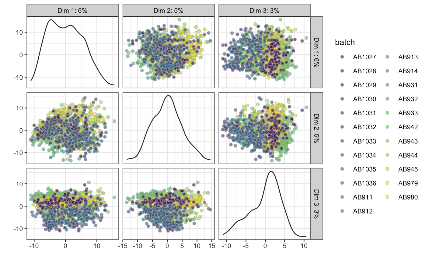
# extract PCs (centered at 0 with runPCA())
PCs4arch = t(reducedDim(hepatocytes, "PCA"))
Fit k=2:8 polytopes to Hepatocytes to find which k best describes the data
# find archetypes
arc_ks = k_fit_pch(PCs4arch, ks = 2:8, check_installed = T,
                   bootstrap = T, bootstrap_N = 200, maxiter = 1000,
                   bootstrap_type = "m", seed = 2543,
                   volume_ratio = "t_ratio", # set to "none" if too slow
                   delta=0, conv_crit = 1e-04, order_type = "align",
                   sample_prop = 0.75)

# Show variance explained by a polytope with each k (cumulative)
plot_arc_var(arc_ks, type = "varexpl", point_size = 2, line_size = 1.5) + theme_bw()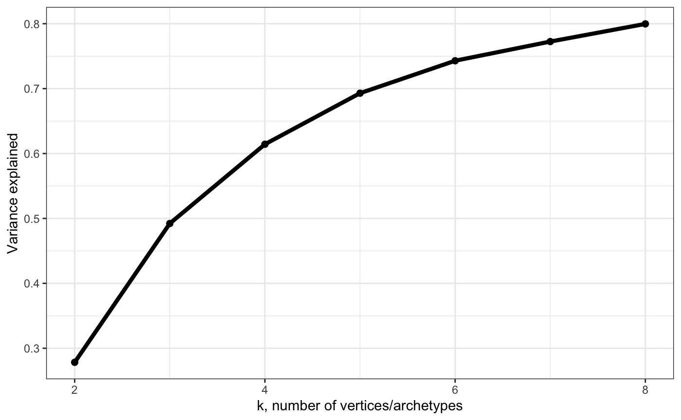
# Show variance explained by k-vertex model on top of k-1 model (each k separately)
plot_arc_var(arc_ks, type = "res_varexpl", point_size = 2, line_size = 1.5) + theme_bw()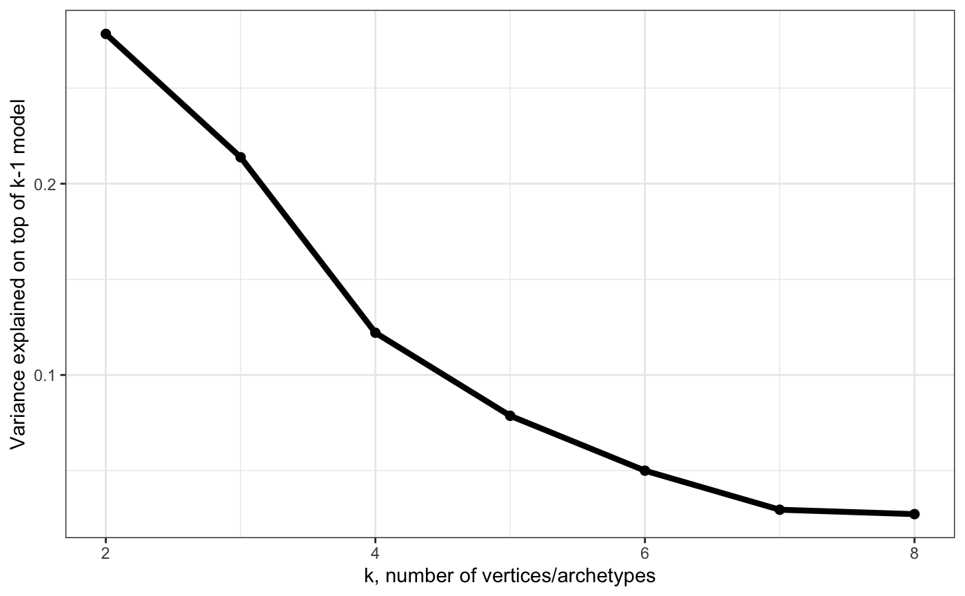
# Show variance in position of vertices obtained using bootstraping
# - use this to find largest k that has low variance
plot_arc_var(arc_ks, type = "total_var", point_size = 2, line_size = 1.5) +
  theme_bw() +
  ylab("Mean variance in position of vertices")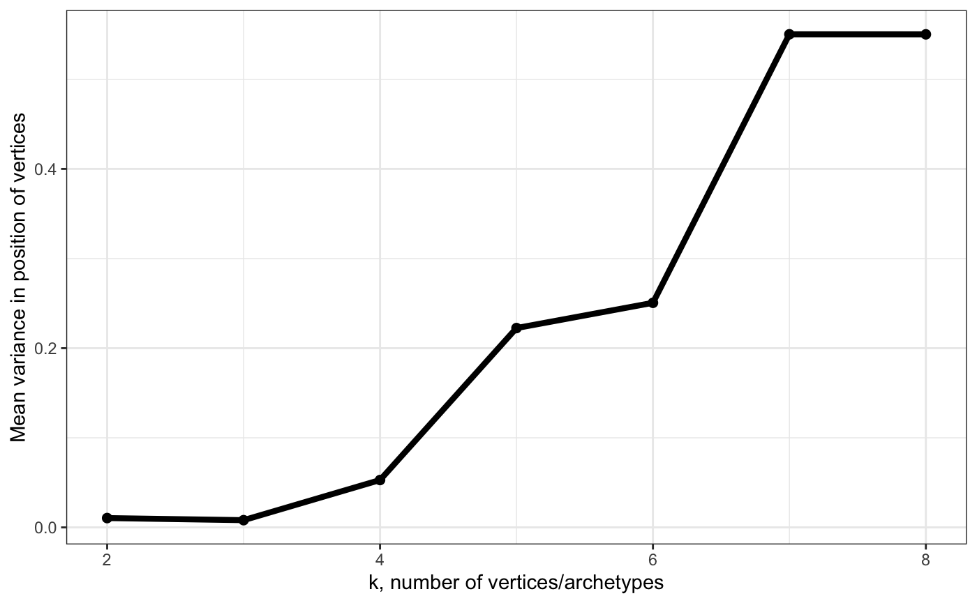
# Show t-ratio
plot_arc_var(arc_ks, type = "t_ratio", point_size = 2, line_size = 1.5) + theme_bw()
## Warning: Removed 1 rows containing missing values (geom_path).## Warning: Removed 1 rows containing missing values (geom_point).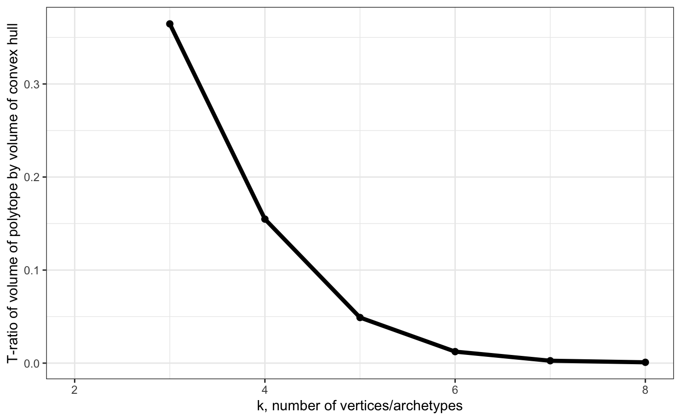
Examine the polytope with best k & look at known markers of subpopulations
Plot show cells in PC space (data = PCs4arch) colored by log2(counts) of marker genes (data_lab = as.numeric(logcounts(hepatocytes[“Alb”,]))). Each red dot is a position of vertex in one of the bootstrapping iterations.
# fit a polytope with bootstraping of cells to see stability of positions
arc = fit_pch_bootstrap(PCs4arch, n = 200, sample_prop = 0.75, seed = 235,
                          noc = 4, delta = 0, conv_crit = 1e-04, type = "m")
p_pca = plot_arc(arc_data = arc, data = PCs4arch,
                 which_dimensions = 1:3, line_size = 1.5,
                 data_lab = as.numeric(logcounts(hepatocytes["Alb",])),
                 text_size = 60, data_size = 6)
plotly::layout(p_pca, title = "Hepatocytes colored by Alb (Albumine)")
p_pca = plot_arc(arc_data = arc, data = PCs4arch,
which_dimensions = 1:3, line_size = 1.5,
data_lab = as.numeric(logcounts(hepatocytes["Cyp2e1",])),
text_size = 60, data_size = 6)
plotly::layout(p_pca, title = "Hepatocytes colored by Cyp2e1")p_pca = plot_arc(arc_data = arc, data = PCs4arch,
which_dimensions = 1:3, line_size = 1.5,
data_lab = as.numeric(logcounts(hepatocytes["Gpx1",])),
text_size = 60, data_size = 6)
plotly::layout(p_pca, title = "Hepatocytes colored by Gpx1")p_pca = plot_arc(arc_data = arc, data = PCs4arch,
which_dimensions = 1:3, line_size = 1.5,
data_lab = as.numeric(logcounts(hepatocytes["Apoa2",])),
text_size = 60, data_size = 6)
plotly::layout(p_pca, title = "Hepatocytes colored by Apoa2")# You can also check which cells have high entropy of logistic regression predictions when classifying all cells in a tissue into cell types. These could have been misclassified by the method and wrongly assigned to Hepatocytes, or these could be doublets.
# find archetypes on all data (allows using archetype weights to describe cells)
arc_1 = fit_pch(PCs4arch, volume_ratio = "t_ratio", maxiter = 500,
noc = 4, delta = 0,
conv_crit = 1e-04)
# check that positions are similar to bootstrapping average from above
p_pca = plot_arc(arc_data = arc_1, data = PCs4arch,
which_dimensions = 1:3, line_size = 1.5,
data_lab = as.numeric(logcounts(hepatocytes["Alb",])),
text_size = 60, data_size = 6)
plotly::layout(p_pca, title = "Hepatocytes colored by Alb")Find genes and gene sets enriched near vertices
# Map GO annotations and measure activities
activ = measure_activity(hepatocytes, # row names are assumed to be gene identifiers
                         which = "BP", return_as_matrix = F,
                         taxonomy_id = 10090, keytype = "ALIAS",
                         lower = 20, upper = 1000,
                         aucell_options = list(aucMaxRank = nrow(hepatocytes) * 0.1,
                                               binary = F, nCores = 3,
                                               plotStats = FALSE))
## snapshotDate(): 2018-10-24## downloading 0 resources## loading from cache
## '/Users/vk7//.AnnotationHub/72903'## Quantiles for the number of genes detected by cell:
## (Non-detected genes are shuffled at the end of the ranking. Keep it in mind when choosing the threshold for calculating the AUC).## min 1% 5% 10% 50% 100%
## 1098.00 1124.23 1259.15 1406.30 2422.50 3976.00## Using 3 cores.## Warning: package 'rngtools' was built under R version 3.5.2## Warning: package 'registry' was built under R version 3.5.2## Using 3 cores.# Merge distances, gene expression and gene set activity into one matrix
data_attr = merge_arch_dist(arc_data = arc_1, data = PCs4arch,
feature_data = as.matrix(logcounts(hepatocytes)),
colData = activ,
dist_metric = c("euclidean", "arch_weights")[1],
colData_id = "cells", rank = F)
# Use Wilcox test to find genes maximally expressed in 10% closest to each vertex
enriched_genes = find_decreasing_wilcox(data_attr$data, data_attr$arc_col,
features = data_attr$features_col,
bin_prop = 0.1, method = "BioQC")
enriched_sets = find_decreasing_wilcox(data_attr$data, data_attr$arc_col,
features = data_attr$colData_col,
bin_prop = 0.1, method = "BioQC")
# Take a look at top genes and functions for each archetype
labs = get_top_decreasing(summary_genes = enriched_genes, summary_sets = enriched_sets,
cutoff_genes = 0.01, cutoff_sets = 0.05,
cutoff_metric = "wilcoxon_p_val",
p.adjust.method = "fdr",
order_by = "mean_diff", order_decreasing = T,
min_max_diff_cutoff_g = 0.4, min_max_diff_cutoff_f = 0.03)## -- archetype_1
##
## Cyp2f2, Hsd17b13, Hsd17b6, Lpin1
## Ly6e, Gc, Fbp1, Dak
## Rpl10, Sds, Hpx, Atp5g1
##
## tricarboxylic_acid_cycle
## citrate_metabolic_process
## tricarboxylic_acid_metabolic_process
##
## -- archetype_2
##
## Cyp2f2, B2m;BC002288, Hsd17b13, Mup3
## Hrsp12, Mug1, Tdo2, Hsd11b1
## Cp, Angptl3, Hal, Cps1
##
## humoral_immune_response_mediated_by_circulating_immunoglobulin
## complement_activation
## aromatic_amino_acid_family_metabolic_process
##
## -- archetype_3
##
## Cyp2e1, Oat, Cyp2a5, Cyp2c29;Cyp2c53-ps
## Cyp1a2, Aldh3a2, Lect2, Ang;Rnase4;2010317E24Rik
## Rgn, Slc22a1, Akr1c6, Gulo
##
## porphyrin_containing_compound_metabolic_process
## response_to_cadmium_ion
## heme_metabolic_process
##
## -- archetype_4
##
## Ptms, Hamp, Rps24, Aes
## Hebp1, Aldh2, Pabpn1, Atf5
## Sec14l2, Stard10, ERCC-00074, Eif4g1
##
## p_pca = plot_arc(arc_data = arc, data = PCs4arch,
which_dimensions = 1:3, line_size = 1.5,
data_lab = activ$ribosomal_large_subunit_biogenesis,
text_size = 60, data_size = 6)
plotly::layout(p_pca, title = "ribosomal_large_subunit_biogenesis activity")## No trace type specified:
## Based on info supplied, a 'scatter3d' trace seems appropriate.
## Read more about this trace type -> https://plot.ly/r/reference/#scatter3d## A marker object has been specified, but markers is not in the mode
## Adding markers to the mode...
## A marker object has been specified, but markers is not in the mode
## Adding markers to the mode...4. Randomise variables to measure goodness of observed fit
To measure goodness of observed fit I compare observed tetrahedron shape to shape of data with no relationships between variables. This is done by comparing the ratio of tertahedron volume to volume of convex hull, a complex shape that contains all of the data. Empirical p-value is fraction of random t-ratios that are at least as high as the observed t-ratio.
# use permutations within each dimension - this is only possible for less than 8 vertices because computing convex hull gets exponentially slower with more dimensions
start = Sys.time()
pch_rand = randomise_fit_pch(PCs4arch, arc_data = arc_1,
                             n_rand = 1000,
                             replace = FALSE, bootstrap_N = NA,
                             volume_ratio = "t_ratio",
                             maxiter = 500, delta = 0, conv_crit = 1e-4,
                             type = "m", clust_options = list(cores = 3))
# use type m to run on a single machine or cloud
# type = "m", clust_options = list(cores = 3))
# use clustermq (type cmq) to run as jobs on a computing cluster (higher parallelisation)
# type = "cmq", clust_options = list(njobs = 10))

# This analysis took:
Sys.time() - start
## Time difference of 2.360313 mins# plot background distribution of t-ratio and show p-value
plot(pch_rand, type = c("t_ratio"), nudge_y = 5)## Picking joint bandwidth of 0.00356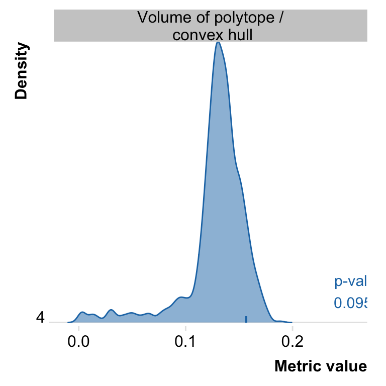
pch_rand## Background distribution of k representative archetypes
## in data with no relationships between variables (S3 class r_pch_fit)
##
## N randomisation trials: 1000
##
## Summary of best-fit polytope to observed data (including p-value):
##
## k var_name var_obs p_value
## 1: 4 varexpl 0.6166675 0.001
## 2: 4 t_ratio 0.1566007 0.095
## 3: 4 total_var NA NaN
##
## varexpl = variance explained by data as weighted sum of archetypes
## t_ratio = volume of polytope formed by archetypes / volume of convex hull
## total_var = total variance in positions of archetypes
## (by bootstraping, mean acrooss archetypes)
##
## Function call:
## randomise_fit_pch(data = PCs4arch, arc_data = arc_1, n_rand = 1000,
## replace = FALSE, bootstrap_N = NA, volume_ratio = "t_ratio",
## maxiter = 500, delta = 0, type = "m", clust_options = list(cores = 3),
## conv_crit = 1e-04)Date and packages used
Sys.Date. = Sys.Date()
Sys.Date.
## [1] "2019-07-09"session_info. = devtools::session_info()
session_info.## ─ Session info ──────────────────────────────────────────────────────────
## setting value
## version R version 3.5.1 (2018-07-02)
## os macOS High Sierra 10.13.6
## system x86_64, darwin15.6.0
## ui X11
## language (EN)
## collate en_GB.UTF-8
## ctype en_GB.UTF-8
## tz Europe/London
## date 2019-07-09
##
## ─ Packages ──────────────────────────────────────────────────────────────
## package * version date lib source
## abind 1.4-5 2016-07-21 [1] CRAN (R 3.5.0)
## annotate 1.60.1 2019-03-07 [1] Bioconductor
## AnnotationDbi * 1.44.0 2018-10-30 [1] Bioconductor
## AnnotationHub 2.14.5 2019-03-14 [1] Bioconductor
## assertthat 0.2.1 2019-03-21 [1] CRAN (R 3.5.1)
## AUCell 1.4.1 2019-01-04 [1] Bioconductor
## backports 1.1.4 2019-04-10 [1] CRAN (R 3.5.2)
## beeswarm 0.2.3 2016-04-25 [1] CRAN (R 3.5.0)
## bibtex 0.4.2 2017-06-30 [1] CRAN (R 3.5.0)
## Biobase * 2.42.0 2018-10-30 [1] Bioconductor
## BiocGenerics * 0.28.0 2018-10-30 [1] Bioconductor
## BiocManager 1.30.4 2018-11-13 [1] CRAN (R 3.5.0)
## BiocNeighbors 1.0.0 2018-10-30 [1] Bioconductor
## BiocParallel * 1.16.6 2019-02-17 [1] Bioconductor
## BioQC 1.10.0 2018-10-30 [1] Bioconductor
## bit 1.1-14 2018-05-29 [1] CRAN (R 3.5.0)
## bit64 0.9-7 2017-05-08 [1] CRAN (R 3.5.0)
## bitops 1.0-6 2013-08-17 [1] CRAN (R 3.5.0)
## blob 1.1.1 2018-03-25 [1] CRAN (R 3.5.0)
## callr 3.3.0 2019-07-04 [1] CRAN (R 3.5.2)
## cli 1.1.0 2019-03-19 [1] CRAN (R 3.5.2)
## codetools 0.2-15 2016-10-05 [2] CRAN (R 3.5.1)
## colorspace 1.4-1 2019-03-18 [1] CRAN (R 3.5.2)
## commonmark 1.7 2018-12-01 [1] CRAN (R 3.5.0)
## cowplot * 0.9.4 2019-01-08 [1] CRAN (R 3.5.2)
## crayon 1.3.4 2017-09-16 [1] CRAN (R 3.5.0)
## crosstalk 1.0.0 2016-12-21 [1] CRAN (R 3.5.0)
## curl 3.3 2019-01-10 [1] CRAN (R 3.5.2)
## data.table * 1.12.2 2019-04-07 [1] CRAN (R 3.5.2)
## DBI 1.0.0 2018-05-02 [1] CRAN (R 3.5.0)
## DelayedArray * 0.8.0 2018-10-30 [1] Bioconductor
## DelayedMatrixStats 1.4.0 2018-10-30 [1] Bioconductor
## desc 1.2.0 2018-05-01 [1] CRAN (R 3.5.0)
## devtools 2.1.0 2019-07-06 [1] CRAN (R 3.5.1)
## digest 0.6.20 2019-07-04 [1] CRAN (R 3.5.2)
## doMC 1.3.5 2017-12-12 [1] CRAN (R 3.5.0)
## doParallel 1.0.14 2018-09-24 [1] CRAN (R 3.5.0)
## doRNG * 1.7.1 2018-06-22 [1] CRAN (R 3.5.0)
## dplyr 0.8.3 2019-07-04 [1] CRAN (R 3.5.2)
## dynamicTreeCut 1.63-1 2016-03-11 [1] CRAN (R 3.5.0)
## edgeR 3.24.3 2019-01-02 [1] Bioconductor
## evaluate 0.14 2019-05-28 [1] CRAN (R 3.5.2)
## foreach * 1.4.4 2017-12-12 [1] CRAN (R 3.5.0)
## fs 1.3.1 2019-05-06 [1] CRAN (R 3.5.2)
## GenomeInfoDb * 1.18.2 2019-02-12 [1] Bioconductor
## GenomeInfoDbData 1.2.0 2018-10-16 [1] Bioconductor
## GenomicRanges * 1.34.0 2018-10-30 [1] Bioconductor
## geometry 0.4.1.1 2019-07-02 [1] CRAN (R 3.5.2)
## ggbeeswarm 0.6.0 2017-08-07 [1] CRAN (R 3.5.0)
## ggplot2 * 3.2.0 2019-06-16 [1] CRAN (R 3.5.2)
## ggridges 0.5.1 2018-09-27 [1] CRAN (R 3.5.0)
## glue 1.3.1 2019-03-12 [1] CRAN (R 3.5.2)
## GO.db 3.7.0 2018-10-25 [1] Bioconductor
## graph 1.60.0 2018-10-30 [1] Bioconductor
## gridExtra 2.3 2017-09-09 [1] CRAN (R 3.5.0)
## GSEABase 1.44.0 2018-10-30 [1] Bioconductor
## gtable 0.3.0 2019-03-25 [1] CRAN (R 3.5.1)
## HDF5Array 1.10.1 2018-12-05 [1] Bioconductor
## htmltools 0.3.6 2017-04-28 [1] CRAN (R 3.5.0)
## htmlwidgets 1.3 2018-09-30 [1] CRAN (R 3.5.0)
## httpuv 1.5.1 2019-04-05 [1] CRAN (R 3.5.2)
## httr 1.4.0 2018-12-11 [1] CRAN (R 3.5.0)
## igraph 1.2.4.1 2019-04-22 [1] CRAN (R 3.5.2)
## interactiveDisplayBase 1.20.0 2018-10-30 [1] Bioconductor
## IRanges * 2.16.0 2018-10-30 [1] Bioconductor
## iterators 1.0.10 2018-07-13 [1] CRAN (R 3.5.0)
## jsonlite 1.6 2018-12-07 [1] CRAN (R 3.5.0)
## knitr 1.23 2019-05-18 [1] CRAN (R 3.5.2)
## labeling 0.3 2014-08-23 [1] CRAN (R 3.5.0)
## later 0.8.0 2019-02-11 [1] CRAN (R 3.5.2)
## lattice 0.20-35 2017-03-25 [2] CRAN (R 3.5.1)
## lazyeval 0.2.2 2019-03-15 [1] CRAN (R 3.5.2)
## limma 3.38.3 2018-12-02 [1] Bioconductor
## locfit 1.5-9.1 2013-04-20 [1] CRAN (R 3.5.0)
## lpSolve * 5.6.13.1 2019-05-28 [1] CRAN (R 3.5.2)
## magic 1.5-9 2018-09-17 [1] CRAN (R 3.5.0)
## magrittr 1.5 2014-11-22 [1] CRAN (R 3.5.0)
## MASS 7.3-50 2018-04-30 [2] CRAN (R 3.5.1)
## Matrix * 1.2-14 2018-04-13 [2] CRAN (R 3.5.1)
## matrixStats * 0.54.0 2018-07-23 [1] CRAN (R 3.5.0)
## memoise 1.1.0 2017-04-21 [1] CRAN (R 3.5.0)
## mime 0.7 2019-06-11 [1] CRAN (R 3.5.2)
## munsell 0.5.0 2018-06-12 [1] CRAN (R 3.5.0)
## ParetoTI * 0.1.11 2019-07-08 [1] local
## pillar 1.4.2 2019-06-29 [1] CRAN (R 3.5.2)
## pkgbuild 1.0.3 2019-03-20 [1] CRAN (R 3.5.1)
## pkgconfig 2.0.2 2018-08-16 [1] CRAN (R 3.5.0)
## pkgdown 1.3.0 2018-12-07 [1] CRAN (R 3.5.0)
## pkgload 1.0.2 2018-10-29 [1] CRAN (R 3.5.0)
## pkgmaker * 0.27 2018-05-25 [1] CRAN (R 3.5.0)
## plotly 4.9.0 2019-04-10 [1] CRAN (R 3.5.1)
## plyr 1.8.4 2016-06-08 [1] CRAN (R 3.5.0)
## prettyunits 1.0.2 2015-07-13 [1] CRAN (R 3.5.0)
## processx 3.4.0 2019-07-03 [1] CRAN (R 3.5.2)
## promises 1.0.1 2018-04-13 [1] CRAN (R 3.5.0)
## ps 1.3.0 2018-12-21 [1] CRAN (R 3.5.0)
## purrr 0.3.2 2019-03-15 [1] CRAN (R 3.5.2)
## R.methodsS3 1.7.1 2016-02-16 [1] CRAN (R 3.5.0)
## R.oo 1.22.0 2018-04-22 [1] CRAN (R 3.5.0)
## R.utils 2.9.0 2019-06-13 [1] CRAN (R 3.5.1)
## R6 2.4.0 2019-02-14 [1] CRAN (R 3.5.2)
## Rcpp 1.0.1 2019-03-17 [1] CRAN (R 3.5.2)
## RCurl 1.95-4.12 2019-03-04 [1] CRAN (R 3.5.2)
## registry * 0.5-1 2019-03-05 [1] CRAN (R 3.5.2)
## remotes 2.1.0 2019-06-24 [1] CRAN (R 3.5.2)
## reshape2 1.4.3 2017-12-11 [1] CRAN (R 3.5.0)
## reticulate * 1.12 2019-04-12 [1] CRAN (R 3.5.2)
## rhdf5 2.26.2 2019-01-02 [1] Bioconductor
## Rhdf5lib 1.4.3 2019-03-25 [1] Bioconductor
## rlang 0.4.0 2019-06-25 [1] CRAN (R 3.5.2)
## rmarkdown 1.13 2019-05-22 [1] CRAN (R 3.5.2)
## rngtools * 1.4 2019-07-01 [1] CRAN (R 3.5.2)
## roxygen2 6.1.1 2018-11-07 [1] CRAN (R 3.5.0)
## rprojroot 1.3-2 2018-01-03 [1] CRAN (R 3.5.0)
## RSQLite 2.1.1 2018-05-06 [1] CRAN (R 3.5.0)
## rstudioapi 0.10 2019-03-19 [1] CRAN (R 3.5.2)
## S4Vectors * 0.20.1 2018-11-09 [1] Bioconductor
## scales 1.0.0 2018-08-09 [1] CRAN (R 3.5.0)
## scater 1.10.1 2019-01-04 [1] Bioconductor
## scran 1.10.2 2019-01-04 [1] Bioconductor
## sessioninfo 1.1.1 2018-11-05 [1] CRAN (R 3.5.0)
## shiny 1.3.2 2019-04-22 [1] CRAN (R 3.5.2)
## SingleCellExperiment * 1.4.1 2019-01-04 [1] Bioconductor
## statmod 1.4.32 2019-05-29 [1] CRAN (R 3.5.2)
## stringi 1.4.3 2019-03-12 [1] CRAN (R 3.5.2)
## stringr 1.4.0 2019-02-10 [1] CRAN (R 3.5.2)
## SummarizedExperiment * 1.12.0 2018-10-30 [1] Bioconductor
## testthat 2.1.1 2019-04-23 [1] CRAN (R 3.5.2)
## tibble 2.1.3 2019-06-06 [1] CRAN (R 3.5.2)
## tidyr 0.8.3 2019-03-01 [1] CRAN (R 3.5.2)
## tidyselect 0.2.5 2018-10-11 [1] CRAN (R 3.5.0)
## usethis 1.5.1 2019-07-04 [1] CRAN (R 3.5.2)
## vipor 0.4.5 2017-03-22 [1] CRAN (R 3.5.0)
## viridis 0.5.1 2018-03-29 [1] CRAN (R 3.5.0)
## viridisLite 0.3.0 2018-02-01 [1] CRAN (R 3.5.0)
## withr 2.1.2 2018-03-15 [1] CRAN (R 3.5.0)
## xfun 0.8 2019-06-25 [1] CRAN (R 3.5.2)
## XML 3.98-1.20 2019-06-06 [1] CRAN (R 3.5.2)
## xml2 1.2.0 2018-01-24 [1] CRAN (R 3.5.0)
## xtable 1.8-4 2019-04-21 [1] CRAN (R 3.5.2)
## XVector 0.22.0 2018-10-30 [1] Bioconductor
## yaml 2.2.0 2018-07-25 [1] CRAN (R 3.5.0)
## zlibbioc 1.28.0 2018-10-30 [1] Bioconductor
##
## [1] /Users/vk7/Library/R/3.5/library
## [2] /Library/Frameworks/R.framework/Versions/3.5/Resources/library